Thursday, June 28, 2012

Secularization in America: part four


Summary so far

In Part One I described trends in market share of major religions in the U.S.: since 1988, the fraction of Protestants dropped from 60% to 51%, and the fraction of people with no religious affiliation increased from 8% to 18%.

In Part Two I used data from the 1988 General Social Survey (GSS) to model transmission of religion from parent to child, and found that the model failed to predict the decrease in Protestants and the increase in Nones that occurred between 1988 and 2010.

In Part Three I looked at changes, between 1988 and 2008, in the spouse tables (which describe the tendencies of people to marry within their religions), the environment table (which describes parents' decisions about their children's religious upbringing), and the transmission table (which describes the likely outcomes for children raised within each religion).  I found that the transmission table has changed substantially since 1988, and accounts for a large part of the observed increase in Nones, but not the decrease in Protestants.

Religiosity curves

Respondents in the GSS are surveyed at different ages, so we can get a sense of when people lose their religion (or acquire one).  I collected all GSS respondents and partitioned them by the religion they were raised in and the decade they were born.  For each of these subgroups, I plotted religiosity (the fraction with some religious preference) as a function of age when surveyed.

Here are the curves for people raised Protestant:


In the top right, we see that people born between 1900 and 1910 and raised Protestant were likely to be religious when they were interviewed in their 70s and 80s.  In the lower left, we see that people born in the 1980s were less likely to be religious when they were interviewed in their 20s.

For the middle generations, we have a better sense of changes in religiosity over a respondent's lifetime.    Several of the curves have an apparent peak in middle age; if this apparent effect is real, the location of the peak may be shifting left.

Overall, these curves are relatively flat, which suggests that respondents are not changing substantially after adulthood (everyone in the GSS is 18 or older).

The curves for Catholics are similar:


Again, there is a substantial differences between generations, but within each generation, little change over the respondents' lifetimes.  People born in the 50s, 60s and 70s might be leaving the church as they age, but it is hard to tell in this plot whether these trends are statistically significant.

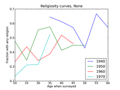
Finally, here are the curves for people raised with no religion:


There are only enough respondents in this category to plot curves for a few generations, and even then, the curves are noisy.  Not surprisingly, people raised without religion are less likely to be religious, and recent generation are less religious than their elders.  Again, the curves are generally flat, suggesting that people generally do not change religious affiliation as adults.

A possible exception is that people born in the 1970s and raised without religion might be finding religion in their 30s.  But this data point is based on a small number of respondents, so it is probably too early to tell.

Why people switch

In 1988 the GSS asked respondents questions about changes in religious affiliation and the reasons for the change.  Unfortunately, it looks like this data won't do me much good, because:

  1. In many cases where a respondent switched from a religious preference to None, they were not asked why.
  2. There are so many inconsistencies in the data, I wonder if it might have been mangled.
  3. Because these questions were only asked once, we can't track trends.
So that's disappointing.


Modeling a mixed-age cohort

One of the challenges of working with GSS data is that the respondents each year are a mixture of people of all ages.  From year to year, the oldest generation drops out of the cohort and the youngest generation joins the mix.

So when there is a trend from each generation to the next, as with religious behavior, there is a lag before the trend appears in a GSS time series, and the slope of the trend is much slower.

However, for purposes of prediction, this lag is actually useful.  For example, 18 years after a baby boom, there is likely to be a spike in college enrollment; that's not really a prediction about the future; it's just a consequence of something that has already happened.


Similarly, we already know what most of the GSS cohort will look like next year.  It will look like the cohort this year, one year older.  The difference is that a few of the oldest respondents are replaced by the next group of 18 year olds.

In the 2010 cohort, the age range is roughly 20-80.  To predict the 2020 cohort, we can:

  1. Remove respondents older than 80.
  2. Age the rest of the respondents by 10 years.
  3. Add a new batch of respondents in their 20s.
Step 2 might be hard if people were changing religious affiliation as they age, but as we saw above, they generally do not.  Step 3 is harder, but there are two reasonable options:
  1. Conservatively, we can assume that the next generation will be like their immediate predecessors.
  2. Alternatively, we can extrapolate from current trends.  This option is probably better for prediction, but in some ways unsatisfying because it does not explain the cause of the trends, or why we should expect them to continue.
If we use this method to predict 20 years into the future, we replace about 25% of the cohort with simulated respondents.  But since 75% of the prediction is based on simple population aging, it is likely to reliable.


Tuesday, June 26, 2012

The falling slinky problem

Let's take a break from statistics and do some physics!

My friend Ted Bunn recently wrote about the falling slinky problem in his blog.  He points to this video, which shows a falling slinky in slow motion.  After the top of the slinky is released, the bottom seems to hover until the top reaches it.  The effect is particularly strange because if you look carefully, the top of the slinky does not accelerate as we expect for an object in free fall.  Rather, it falls at a constant rate.

Ted explains:
...the information that the top end has been dropped can’t propagate down the slinky any faster than the speed of sound in the slinky (i.e., the speed at which waves propagate down it), so there’s a delay before the bottom end “knows” it’s been dropped. But it’s surprising (at least to me) to see how long the delay is.
This explains why there is a delay, but to me it doesn't explain why the delay is the same as the time it takes for the top of the slinky to reach the bottom.  There are lots of models out there that explain parts of this behavior, but the ones I found are either complicated or wrong.

Here's my take on it.  First, let's assume that what we see in the video is correct: the slinky collapses from top to bottom, so that each coil doesn't move until the one above it comes down and (nearly) hits it.

Let's call the initial length L and the mass m.  After some time, a fraction of the slinky, x, has collapsed.  At that point, the collapsed part of the slinky has mass xm at height (1-x)L.  The rest of the slinky is spread uniformly [EDIT: this assumption is not right...see Ted's comment below] between height 0 and (1-x)L.  So the center of mass is

x(1-x)L + (1-x)(1-x)L/2

Since the slinky is in free fall, we know the center of mass as a function of time:

L/2 - g/2 t^2

If we set those equal and type them into WolframAlpha, we get

x = sqrt(g/L) t

Which means that the top of the slinky is moving at constant speed.  Remember that x is the fraction of the slinky that collapsed; to get the distance traveled, we multiply by L:

d = xL = sqrt(gL) t

So the speed of the top of the slinky is sqrt(gL).

We can get to the same result a different way by using the formula for wave speed in a vibrating string: sqrt(T/μ), where T is tension and μ is mass per linear measure.  In this case T=mg and μ=m/L.  Plug that in and get wave speed sqrt(gL).

I think this analysis is useful, but to be rigorous, I haven't really explained why the slinky behaves the way it does.  I have only shown that if the slinky collapses from top to bottom (as it appears to), then the top moves at a constant speed (as it appears to).


[UPDATE: Provoked by my amateurish attempts at Physics, Ted Bunn wrote up a version of this model that deals correctly with the change in the density of the spring from top to bottom.  The result is that the speed of the top of the slinky is almost constant -- it slows down a bit at the end. ]


Friday, June 22, 2012

Secularization in America: part three

In Part One I described trends in market share of major religions in the U.S.: since 1988, the fraction of Protestants dropped from 60% to 51%, and the fraction of people with no religious affiliation increased from 8% to 18%.

In Part Two I used data from the 1988 General Social Survey (GSS) to model transmission of religion from parent to child, and found that the model failed to predict the decrease in Protestants and the increase in Nones that occurred between 1988 and 2010.

I proposed several reasons the model might have failed:

  1. The spouse tables are based on the parents of 1988 respondents.  People from later generations might be increasingly likely to marry outside their religion.
  2. The environment table is also based on the previous generation; again, later parents might be making different decisions about the religious environment of their children.
  3. The transmission table is based on 1988 respondents; it's possible that after 1988, children were less likely to adopt the religion they were raised in.  Anecdotally, the culprits most often blamed for this effect are college and the Internet.
  4.  Finally, I have not considered adult conversions from one religious identity to another.  The GSS has data on these switches, so I could add them to the model.
I will investigate each possibility in turn, starting with the prevalence of mixed-religion marriages.  In Secularization, Steve Bruce presents results from a study of intermarriage in the UK that found that the rate of vertical transmission:
 "is halved if the parents are of different faiths (even when the differences are just Methodist-Anglican).  Even if the parents agree on which faith they wish to pass on, the fact of disagreement makes the child aware that there are good people in other churches and introduces the relativism that weakens conviction. [page 71]"
So if the rate of mixed marriages is increasing, that could contribute to the increasing number of Nones. 
To measure this effect, I used these GSS variables:
  • RELIG: What is your religous preference?
  • SPREL: What is your husband's/wife's religious preference?
In cases where one partner converts to the other's religion before marriage, that would count (for this model) as a same-religion marriage, since we are interested in the decision the couple makes about the religious environment they raise children in.


The Spouse Tables

The following graph shows the fraction of same-religion marriages over the history of the survey (data for SPREL were not collected every year):


Before 1988, the fraction of same-religion marriages was around 84%; after 1988 it fell to 78%.  The abruptness of the change makes me worry that it may be an artifact; for example, a chance in the wording of the question.  Also, these results only include respondents who are married, so they are biased toward older people and socio-economic groups that are more likely to be married.

But as it turns out, even if we take the data at face value, it has a small effect on the model's predictions.
I used the respondents from 2004-2010 to build spouse tables for men and women (see Part Two), then ran the 1988 model again with the anachronistic data.  The results are almost identical to what we saw last time:

The only noticeable effect is that the prediction for Other got worse.  I conclude:
  1. It's possible that people are more likely now to marry outside their religion than in 1988, but the difference is small, and
  2. Even if we cheat by using the 2004-2010 data in 1988, this change does not explain the subsequent changes in the fractions of Protestants and Nones.

The Environment Table

It seems unlikely that parents now are making different decisions about what religious environment to raise their children in, but just to rule it out, I compared the environment tables for 1988 and 2008.

prot cath jew other none    change  N       excess
prot-prot 97 1 0 0 2 +1 634 8.7
prot-cath 43 46 0 1 10 +4 49 1.9
prot- jew 0 0 0 0 0 +0 1 0.0
prot-othe 44 21 0 36 0 +0 5 0.0
prot-none 85 4 0 0 11 +5 90 4.2
cath-prot 30 56 0 0 14 +14 37 5.1
cath-cath 1 98 0 0 1 +0 294 0.8
cath- jew 0 0 0 0 0 +0 0 0.0
cath-othe 0 0 0 0 0 +0 2 0.0
cath-none 2 82 0 0 16 +7 20 1.5
 jew-prot 0 0 0 0 0 +0 1 0.0
 jew-cath 0 100 0 0 0 +0 0 0.0
 jew- jew 0 0 96 0 4 +0 27 0.0
 jew-othe 0 0 0 0 0 +0 0 0.0
 jew-none 0 0 67 0 33 +33 0 0.0
othe-prot 27 0 0 54 18 +18 4 0.7
othe-cath 0 43 0 57 0 +0 3 0.0
othe- jew 0 0 0 0 0 +0 0 0.0
othe-othe 7 0 0 84 9 +3 28 0.7
othe-none 25 25 0 25 25 +25 4 1.0
none-prot 83 0 0 0 17 +17 6 1.0
none-cath 14 68 0 0 18 -82 2 -1.6
none- jew 0 0 100 0 0 +0 0 0.0
none-othe 0 0 0 0 0 -100 1 -1.0
none-none 23 4 0 0 74 +18 34 6.1

The left column is the mother's-father's religion.  The next five columns show the religious environments those parents chose, as reported by their children in 2008.  For example, the second row shows that if the mother is Protestant and the father Catholic, 43% of the children were raised Protestant, 46% Catholic, and 10% None.

The next column shows the change in the None column, in percentage points, since the 1988 survey.  N is the number of families in 1988 that fell into each category.  Finally, Nones is the product of change and N, an estimate of the number of additional Nones in the 1988 survey that could be explained by changes in the environment table.  The total of this column is 29, which is not nearly enough to explain the actual excess of 177.

Of course, most of the numbers in the change column are based on small samples, so we should not take them too seriously.  By running simulations with resampled survey data, we can take account of these sample sizes.

Using the tables from 1988 to predict the fractions of Nones in 2008, we expect only 8.0% (compared to the actual 16.8%).  If we used the environment table from 2008, the prediction goes to 8.5%.  If we also use the spouse table, it goes up to 8.7%.  So clearly the changes in these tables were not enough to explain the observed changes.

The transmission table

The transmission table is a cross-tabulation of the religion the respondent was brought up in and the religion reported when surveyed.  It shows the outcome, after some years, of parents' decisions about their children's religious upbringing and the effect of the environment.

The following is the transmission table for 2008, with changes since 1988:


prot cath jew other none change  N       excess
prot 82 3 1 2 13 +7 951 67.7
cath 17 70 0 2 12 +6 414 24.6
jew 9 2 73 1 14 +9 31 2.7
other 12 2 0 75 10 +1 31 0.4
none 31 5 1 2 62 +5 53 2.6

Each row corresponds to a religious upbringing; each column shows a possible outcome.  For example, the first row shows that of children raised Protestant, 82% report that their religious preference is Protestant, and 13% report None.  The fraction of Nones has increased 7 percentage points since 1988. Since there are 951 people in this row, this increase accounts of 68 excess Nones in the 2008 survey.

Overall, the changes in the transmission table account for 98 excess Nones, which is a little more than half of the observed increase.

If we run the simulations again, applying the transmission table from 2008 in 1988, we get the following predictions:
The prediction for Nones is better, but it's clear that this model still misses the mark: it predicts that the fraction of Catholics should be going down, and fails to predict the decrease in the fraction of Protestants.

The problem is that I am treating everyone interviewed in 1988 as a cohort, but they represent people of all ages, who were raised in different environments.  Also, I am using data from 2008 to predict what will happen in 2008, so I have got away from the original goal, to see whether the changes that occurred between 1988 and 2008 could have been predicted in 1988.

However, this model has given me some leads.  It looks like a large part of the increase in Nones is due to changes in the transmission table, possibly a small part due to the environment table, and little or none due to the spouse tables.

Next time I will present a different model that reorganizes respondents into cohorts by age of birth, which will make it possible to compare people raised over the same time span.  It will also allow me to look for trends that began prior to 1988.


Thursday, June 21, 2012

Secularization in America: part two

In Part One I described some trends in market share of the major religions in the U.S.; in particular, since 1988, the fraction of Protestants dropped from 60% to 51%, and the fraction of people with no religious affiliation increased from 8% to 18%.

I would like to know if something happened after 1988 to cause these changes, or if they could have been predicted based on patterns occurring before 1988.  As a first step, I will use data from 1988 to model vertical transmission (from parent to child) and see if it predicts the observed changes

My model of vertical transmission works like this:

  • Each respondent chooses a spouse,
  • Each pair decides what religion to bring their children up in,
  • Each child chooses a religion.
I model each step of this process using data from the General Social Survey (GSS); specifically, I used these variables.

  • RELIG: What is your religous preference?
  • RELIG16: In what religion were you raised?
  • MARELIG: What was your mother's religious preference when you were growing up?
  • PARELIG: What was your fathers's religious preference when you were growing up?
The first two questions were asked every year, but questions about parents' religion were only asked in 1988 and 2008.  I will use the data from 1988 to build and validate models, then use the data from 2008 to make predictions.

I used MARELIG and PARELIG to build two "Spouse tables", one for men and one for women.  Here is the table for men:

Spouse Table (men)

prot cath jew other none
prot 93 6 0 0 1
cath 14 85 0 0 1
jew 4 0 96 0 0
other 6 4 0 90 0
none 59 13 0 3 24

Each row indicates the religion of a male respondent; each column is the religion of a possible spouse; the numbers are percents.  For example, the first row indicates that 93% of male Protestants married other Protestants, and another 6% married Catholics.

Here is the spouse table for women:

Spouse Table (women)

prot cath jew other none
prot 82 7 0 0 12
cath 10 85 0 0 5
jew 4 0 96 0 0
other 8 3 0 74 15
none 13 7 0 0 80

In general, women are more likely to marry out of their religion than men, but still the great majority marry a co-religionist.  One asymmetry is apparent: men with no religion seldom marry another None (24%), but women with no religion usually do (80%).  This effect is partly due to the gender gap: 11% of male respondents are Nones, but only 5% of the women are (there is a similar, possibly smaller, gender gap in the CIRP data).

Once the respondents have paired up, they decide what religion to raise the children in.  The following table shows results from the 1988 data.  The rows enumerate all pairs of mother's and father's religion; the columns indicate the religious environment they chose.  For example, the second row indicates that if a Protestant woman marries a Catholic man, they raise the children Protestant 58% of the time, Catholic 36% of the time, and None 6%.

Environment table

parents prot cath jew other none
prot-prot 99 1 0 0 1
prot-cath 58 36 0 0 6
prot-jew 100 0 0 0 0
prot-other 100 0 0 0 0
prot-none 89 4 0 1 7
cath-prot 39 61 0 0 0
cath-cath 1 99 0 0 0
cath-jew 0 0 0 0 0
cath-other 100 0 0 0 0
cath-none 17 69 0 6 8
jew-prot 0 0 100 0 0
jew-cath 0 0 0 0 0
jew-jew 0 0 96 0 4
jew-other 0 0 0 0 0
jew-none 0 0 0 0 0
other-prot 60 0 0 40 0
other-cath 0 0 0 100 0
other-jew 0 0 0 0 0
other-other 7 2 0 89 2
other-none 33 0 0 67 0
none-prot 100 0 0 0 0
none-cath 0 0 0 0 100
none-jew 0 0 0 0 0
none-other 0 0 0 0 0
none-none 40 4 0 0 56


One surprise in this table is the last row: when two people with no religion marry, 40% of the time they apparently choose to raise their children Protestant.  This seems unlikely, but there are several possible explanations: (1) the parents might have chosen to raise their children in the prevalent religion of their community, (2) a respondent might not have been raised by his parents, (3) a respondent might not be reporting his parents' religion accurately.  For purposes of modeling I take these responses at face value.


Children raised with a religion usually adopt that religion, but not always.  The following "transition table" shows possible outcomes for each religious environment.  For example, 89% of respondents who say they were raised Protestant also report that their religious preference is Protestant, but 3% are Catholic and 6% have no religious preference.  More people convert from Catholic to Protestant than the other way around.

Transition table

prot cath jew other none
prot 89 3 0 1 6
cath 11 83 0 0 6
jew 0 0 95 0 5
other 5 3 0 83 9
none 32 11 0 0 57

As expected, the majority of people raised with no religion report no religious preference, but 32% of them identify as Protestant and 11% identify as Catholic.  I found that surprising.  I will look more closely later, but for now, again, I will take it at face value.

Finally, we can combine these results into a single "Generation table" that shows the transitions from one generation to the next.  I ran simulations with following steps.

  • For each respondent, choose a spouse's religion from the Spouse Table.
  • For each parent pair, choose a religious environment from the Environment Table.
  • For each hypothetical child, choose a religious identity from the Transition Table.
  • For each parent-child pair, make an entry in the Generation Table, below. 

Since this computation is based on random simulations, it varies from run to run, but here is a typical outcome:

Generation table

prot cath jew other none
prot 86 6 0 1 7
cath 19 72 1 1 7
jew 0 0 95 0 5
other 29 10 0 55 6
none 67 9 0 1 23

Assuming that a generation time is about 22 years, we can use this model to predict the distribution of religions in 2010 (using only data from 1988).  This figure shows the actual time series and the model predictions for each group:

On the right side of the plot, the vertical lines show the 90% confidence interval; the boxes show the mean of 20 simulation runs.  [One technical note: each simulation is based on tables from resampled survey data, so the confidence intervals reflect both the sampling error of the survey and random variation of the simulations.]

The actual values for Catholics, Jews and Other fall within the prediction intervals, but the model fails to predict the decrease in Protestants or the increase in None.

So, what's missing from this model that could account for the observed changes?
  1. The spouse tables are based on the parents of 1988 respondents.  People from later generations are increasingly likely to marry outside their religion.
  2. The environment table is also based on the previous generation; again, later parents might be making different decisions about the religious environment of their children.
  3. The transition table is based on 1988 respondents; it's possible that after 1988, children were less likely to adopt the religion they were raised in.  Anecdotally, the culprits most often blamed for this effect are college and the Internet.
  4.  Finally, I have not considered adult conversions from one religious identity to another.  The GSS has data on these switches, so I could add them to the model.
Over the next few installments, I will investigate each of these factors to see which, if any, account for the observed changes.


Tuesday, June 19, 2012

Secularization in America, part one.

In the last year or so I have written several articles about trends in religion among college students:

  1. Are religious colleges getting more religious?
  2. Freshman hordes more godless than ever!
  3. Freshman hordes even more godless!
All of these are based on data from the Cooperative Institutional Research Program (CIRP) which runs the Freshman Survey, an annual survey of more than 200,000 incoming students at 270 colleges and universities in the U.S.

More recently, I read Secularization: In Defence of an Unfashionable Theory, by Steve Bruce.  Bruce presents the "unfashionable theory" that as societies modernize, they secularize.  In his formulation, modernization includes trends toward individualism, industrial capitalism, science and technology; and secularization means "decline in the social significance of religion."

The poster child for secularization is Western Europe, where the social influence of religion has been in decline for centuries, and where in every country the fraction of people with no religious affiliation has been increasing for decades.

But skeptics have suggested that countries where people are still religious, like the United States and many countries in the Middle East, are exceptions that disprove the theory.  Bruce replies that religious countries in the Middle East are not exceptions because they are not modern, and the United States is not an exception because it is, in fact, secularizing.

The data from the Freshman Survey are consistent with secularization.  The number of incoming college students with no religious affiliation has been climbing consistently since 1978, and the number of students reporting participation in religious service has fallen at about the same rate.

Of course, college students are not a random sample of the population; for that, we can use data from the General Social Survey (GSS), which is (according to the GSS) "widely regarded as the single best source of data on societal trends."  It has run since 1972; each year (or every other year since 1994) it surveys a sample of about 2000 adults randomly sampled from the U.S. population.  Respondents answer hundreds of questions about their background, life history, and beliefs.  Many questions are repeated from year to year for trend analysis.

I will use this dataset to answer several questions:
  1. Is there evidence of secularization in the U.S. (Hint: yes).
  2. Can we explain the causes?
  3. Can we predict how these trends will continue over the next few decades.
To get started, I tracked responses to the question, "What is your current religious preference?"  The original set of options was Protestant, Catholic, Jewish, some other religion, or no religion.  After 1994, the set of options was expanded, but for my purposes the original options are enough to describe large-scale trends.  The following graph shows the fraction of the population in each group over time.

A few trends are apparent: the percentage of Protestants is declining; the percentages of Other and None are increasing.  These trends are clearer in the following figures, broken into two intervals:

From 1972 to 1988, the fraction of Protestants and Catholics was unchanged, but the fraction of Nones may have increased.
From 1988 to 2010 (the most recent survey year), the fraction of Protestants and Jews declined, and the fraction of Nones increased by almost 250%.  The number of Others increased during both intervals, with more variability.

This dataset shows signs of secularization in the U.S., at least since 1972.  But religious affiliation is just one aspect of religious identity; there is a lot more data in the GSS to look at.

My particular interest is in explaining the trends we have seen so far, and predicting what's coming next.  It is tempting to think that something happened in 1988 to cause the inflections in these curves, but I think it is more likely that the origin of these changes goes back farther.  

To test that idea, let's pretend that it's 1988.  We have see some changes in the market share of different religions since 1972, but nothing bigger than a few percentage points, and no indication of acceleration.  Could we have predicted the much larger changes coming between 1988 and 2010?

In the next few articles, I develop several models intended to answer that question.  Then I turn to prediction: using the data up to 2010 (and 2012 when it is available) what can we expect in the next 20 years?