Bayesian predictions for Super Bowl XLIX
Bayesian analysis of match rates on Tinder
Bayesian survival analysis for Game of Thrones
Now, with the Boston Marathon coming up, we have an article about predicting world record marathon times.
Modeling Marathon Records With Bayesian Linear Regression
Cypress Frankenfeld
In this blog article, Allen Downey shows that marathon world record times have been advancing at a linear rate. He uses least squares estimation to calculate the parameters of the line of best fit, and predicts that the first 2-hour marathon will occur around 2041.
I extend his model, and calculate how likely it will be that someone will run a 2-hour marathon in 2041. Or more generally, I find the probability distribution of a certain record being hit on a certain date.
I break down my process into 4 steps:
- Decide on a set of prior hypotheses about the trend of marathon records.
- Update my priors using the world record data.
- Use my posterior to run a monte-carlo simulation of world records.
- Use this simulation to estimate the probability distribution of dates and records.
What are my prior hypotheses?
Since we are assuming the trend in running times is linear, I write my guesses as linear functions,
yi(xi) = α + βx + ei ,
where α and β are constants and ei is random error drawn from a normal distribution characterized by standard deviation σ. Thus I choose my priors to be list of combinations of α, β, and σ.
intercept_estimate, slope_estimate = LeastSquares(dates, records)
alpha_range = 0.007
beta_range = 0.2
alphas = np.linspace(intercept_estimate * (1 - alpha_range),
intercept_estimate * (1 + alpha_range),
40)
betas = np.linspace(slope_estimate * (1 - beta_range),
slope_estimate * (1 + beta_range),
40)
sigmas = np.linspace(0.001, 0.1, 40)
hypos = [(alpha, beta, sigma) for alpha in alphas
for beta in betas for sigma in sigmas]
I set the values of α, β, and σ partially on the least squares estimate and partially on trial and error. I initialize my prior hypotheses to be uniformly distributed.
How do I update my priors?
I perform a bayesian update based on a list of running records. For each running record, (date, record_mph), I calculate the likelihood based on the following function.
def Likelihood(self, data, hypo):
alpha, beta, sigma = hypo
total_likelihood = 1
for date, measured_mph in data:
hypothesized_mph = alpha + beta * date
error = measured_mph - hypothesized_mph
total_likelihood *= EvalNormalPdf(error, mu=0, sigma=sigma)
return total_likelihood
I find the error between the hypothesized record and the measured record (in miles per hour), then I find the probability of seeing that error given the normal distribution with standard deviation of σ.
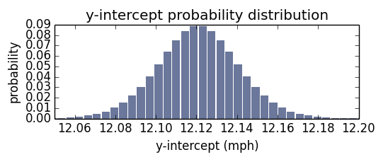
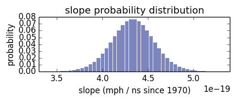
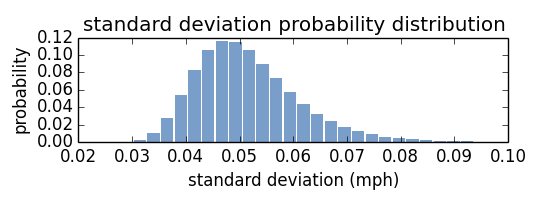
The posterior PMFs for α, β, and σ
 |
α
|
 |
β
|
 |
σ
|
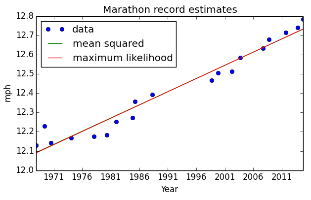
Here are the posterior marginal distributions of α, β, and σ after updating with all the running records. The distributions of α and β peak close to the least squares estimate. How close are they to least squares estimate? Here I’ve plotted a line based on the maximum likelihood of α, β, compared to the least squares estimate. Graphically, they are almost indistinguishable.
But I use these distributions to estimate more than a single line! I create a monte-carlo simulation of running records.
How do I simulate these records?
I pull a random α, β, and σ from their PMF (weighted by probability), generate a list of records for each year from 2014 to 2060, then repeat. The results are in the figure below, plotted alongside the previous records.
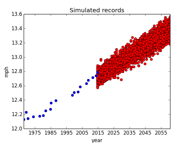
It may seem counterintuitive to see simulated running speeds fall below the current records, but it make sense! Think of those as years wherein the first-place marathon didn’t set a world-record.
These simulated records are most dense where they are most likely, but the scatter plot is a poor visualization of their densities. To fix this, I merge the points into discrete buckets and count the number of points in each bucket to estimate their probabilities. This resulting joint probability distribution is what I’ve been looking for: given a date and a record, I can tell you the probability of setting that record on that date. I plot the joint distribution in the figure below.
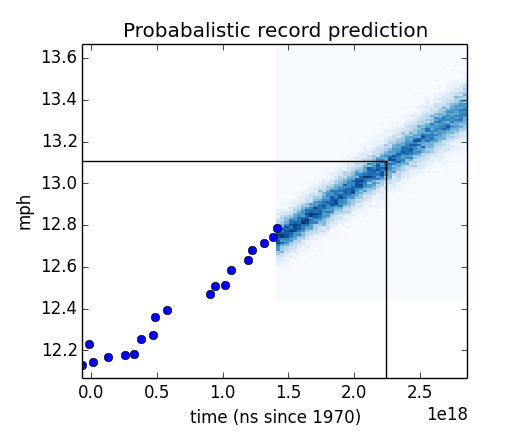
It is difficult to create a pcolor plot with pandas Timestamp objects as the unit, so I use nanoseconds since 1970. The vertical and horizontal lines are at year 2041 and 13.11mph (the two-hour marathon pace). The lines fall within a dense region of the graph, which indicates that they are likely.
To identify the probability of the two-hour record being hit before the year 2042, I take the conditional distribution for the running speed of 13.11mph to obtain the PMF of years, then I compute the total probability of that running speed being hit before the year 2042.
>>> year2042 = pandas.to_datetime(‘2042’)
>>> joint_distribution.Conditional(0, 1, 13.11).ProbLess(year2042.value)
0.385445
This answers my original question. There is a 38.5% probability that someone will have run a two-hour marathon by the end of 2041.
To get a bigger picture, I create a similar conditional PMF for each running speed bucket, convert it to a CDF, and extract the years corresponding to several percentiles. The 95th percentile means there is a 95% probability of reaching that particular running speed by that year. I plot these percentiles to get a better sense of how likely any record is to be broken by any date.
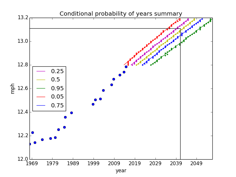
Again, the black horizontal and vertical lines correspond to the running speed for a two-hour marathon and the year 2041. You can see that they fall between 25% and 50% probability (as we already know). By looking at this plot, we can also say that the two-hour marathon will be broken by the year 2050 with about a 95% probability.
No comments:
Post a Comment